A Colorful Hilbert Something or Other

A nice image from the Ogre's Gallery.

C0, C1, and C2 functions

From Wikipedia's Smooth Functions:

"The class C0 consists of all continuous functions. The class C1 consists of all differentiable functions whose derivative is continuous; such functions are called continuously differentiable."

A differentiable function might not be C1. The function f(x) = x^2*sin(1/x) for x \neq 0 and f(x) =0 for x=0 is everywhere continuous and differentiablem, but its derivative is f'(x) = -cos(1/x) + 2x*sin(1/x) for x \neq 0 and f'(x) =0 for x=0, which is discontinuous at x=0, so it is not C1.

The Weirstrass Function

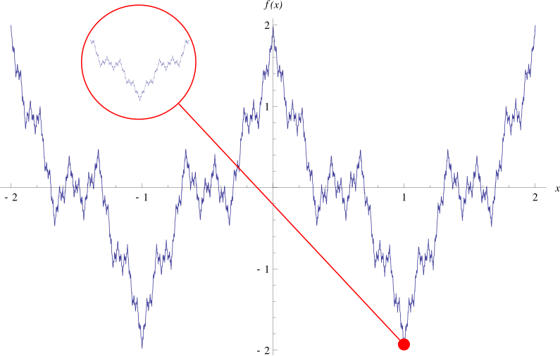The Weierstrass Function

From Wikipedia's Weirstrass Function comes this good graphic of an everywhere continuous but nowhere differentiable function.




Nov. 9. I wondered about the following questions:

Do there exist monotonic functions that are everywhere continuous but nowhere differentiable?

Do there exist monotonic functions that are nowhere continuous?

No in either case, it seems. Here is an answer:

First, monotone functions only can have a countable number of discontinuities (since these must be jump discontinuities where the function makes progress upward/downward and all uncountable positive sums are infinite).

Moreover, for a more involved reason, the set of points where a monotone function is not differentiable must have lebesgue measure 0. (I.e. they are differentiable almost everywhere.)

One way to see this is from the fact that for an increasing function the limit of the slope of the secant line between (x,f(x)) and (x+h,f(x+h)) for each fixed x as h varies must always exist (and be nonnegative), provided we allow it to also take on the value +infinity. Then one can show this cannot be infinity except on a measure 0 set...again, the function would make too much progress.

On the other hand, the derivative can not exits on an uncountable set (e.g. the Cantor staircase function). Moreover, there is a slightly more sophisticated example of a strictly increasing continuous function that goes from f(0)=0 to f(1)=1 which has a derivative equal to 0 almost everywhere, in fact whenever the derivative exists.

Since they are differentiable almost everywhere, the derivatives of monotone functions are Lebesgue integrable functions (extend to the nondifferentiable points however you want, it won't affect the integral). So the previous example shows that the Fundamental Theorem of Calculus cannot be extended to even the class of derivatives of continuous monotone functions (even when the resulting derivative function is the constant function), since then we would have 0=\int_01 f'(x)dx=f(1)-f(0)=1. (The FTC does work, however, if f is continuous and the derivative exists except at a countable set).

From PlanetMathm here is Cantor's Staircase (in a 20-iteration figure, instead of infinite iterations), which uses a Cantor Set to build a function which is continuous and monotonic (strictly?) but with f'(x) =0 almost everywhere.

Graph of the cantor function using 20 iterations

Quasiconcavity

Martin Osborne has some good notes on quasiconcavity. I'm still not satisfied, though. It's a basic enough idea that I wish I had better intuition for it, and lots and lots of pictures of functions that are or are not quasiconcave.

October 25: Here are some key features of a quasiconcave function f(x).

• It has convex upper level sets. The set of points x such that f(x) >= a is convex for any number a.
• It has convex indifference curves if it is a utility function. If f(x) is strictly monotonically increasing, the function g(x) such that f(x)=a is a convex function.

Every concave function is quasiconcave, but some quasiconcave functions are not concave. A key feature of quasiconcavity that concavity doesn't have is that if you do an increasing transformation of a qc function, it is still qc. I wonder if the following is true:

Conjecture: Iff function f(.) is quasiconcave, there exists an increasing transformation g(.) such that g(f(.)) is concave.

I'd start to prove the conjecture this way. Let x and y be points in the upper level set of f(.), which means f(x)>=a and f(y)>=a. Since f(.) is quasiconcave, the upper level set is convex, which means that f(mx+ (1-m)y) >=a too. What we need to show first is that there exists some increasing function g() such that
g(f(mx+ (1-m)y)) >= mg(f(x)) + (1-m)g(f(y)). I think we need to start by assuming that f(x) \neq f(y), and that they are both on the boundary of that convex upper level set. Then we can see how g has to affect those two levels of f differently.

If the conjecture is true, then maybe we can think of quasiconcavity as being the equivalent of concavity for functions that are just defined on ordinal, not cardinal spaces.

October 26. Why, though, do we worry about quasi-concavity at all in economics? Why not just assume that utility functions are concave? The conventional answer would be that utility is ordinal, not cardinal. That is a bad answer for three reasons. First, even if it is ordinal, we could say, "It's only the ordinal properties of a utility function that affect decisions. Therefore, for convenience, let's say that whatever function you start with, you have to use a monotonic transformation to make it concave before we start working with it." Second, we might say, "Since only ordinal properties matter, let's assume utility is concave for convenience." Third, we might accept cardinality. Everybody uses von-Neumann Morgenstern cardinal utility in their models anyway, making only a brief nod, if any, to ordinality. But a risk-averse agent has concave utility. For these reasons, I wonder why it's worth making our graduate students learn about quasi-concavity. The opportunity cost is that they're not learning about something more useful such as the CAPM or the Coase Theorem.

Maybe quasi-concavity comes up in enough other contexts to be important. I know Rick Harbaugh has a paper on comparative cheap talk where it comes up. In Varian, it comes up first in production functions, where it allows you to have convex input sets for a given output without requiring diminishing returns to scale, as true concavity would.

October 27. Yet another thought. Margherita Cigola has done work on defining quasiconcavity in ordinal spaces, on lattices. Convexity has to be defined specially there. She uses a different (equivalent in R space) definition of quasiconcavity:
f(mx + (1-m)y) >= mf(x) + (1-m)f(y)

I like that because it is closer to the definition of concavity.

Or another, suitable when the function is differentiable: f is quasiconcave if whenever there is a maximum (i.e., the first derivatives are zero), the matrix of second derivatives is negative definite. MR suggested that, for the single-dimensional x case. I'm not sure it does generalize that way.

Significant Figures

I haven't used this idea since high school, really, but it comes up now and then, so I looked it up in Wikipedia. 100 has one significant figure, as do 20 and 23 and .0001, the article says. The number .00200, however, has three significant figures. The number 1.234 has 4 significant figures. Digits beyond accurate measurement don't count as significant. There is ambiguity, however, in whether 100 feet really has just one significant figure. It may be that you have measured it to the nearest foot, in which case it really has three significant figures.

The real importance of significant figures comes in doing arithmetic. If you run 100 yards in 11.71 seconds, and the 100 has three significant figures, then the speed should be written with three significant figures as 8.54 yards per second, not as 8.53970965 yards per second.

Reuleaux Triangle

This Reuleaux Triangle from Wolfram/Mathematica is a nice idea for a shape. It is the shape a Wankel engine takes, perhaps because you can rotate this triangle inside a square as shown at the Wolfram site.

Some Math Graphics

Dean Anton Sherwood has lots of good math graphics at http://www.ogre.nu/doodle/#chainmail. Here's one.

Annulus

An annulus is the region lying between two concentric circles in 2-space-- a ring.

Lipschitz continuity

From Wikipedia:

...Lipschitz continuity, named after Rudolf Lipschitz, is a smoothness condition for functions which is stronger than regular continuity. Intuitively, a Lipschitz continuous function is limited in how fast it can change; a line joining any two points on the graph of this function will never have a slope steeper than a certain number called the Lipschitz constant of the function....

* The function f(x) = x^2 with domain all real numbers is not Lipschitz continuous. This function becomes arbitrarily steep as x goes to infinity. It is however locally Lipschitz continuous.

* The function f(x) = x^2 defined on [ − 3,7] is Lipschitz continuous, with Lipschitz constant K = 14.

Elasticities in Regressions. (update of old post)Here are how to calculate elasticities from regression coefficients, a note possibly useful to economists who like me keep having to rederive this basic method:

1. The elasticity is (%change in Y)/(%change in X) = (dy/dx)*(x/y).
2. If y = beta*x then the elasticity is beta*(x/y).
3. If y = beta* log(x) then the elasticity is (beta/x)*(x/y) = beta/y.
4. If log(y) = beta* log(x) then the elasticity is (beta*y/x)*(x/y) = beta, which is a constant elasticity.
   (reason: then y= exp(beta*log(x)), so dy/dx = beta*exp(beta*log(x))*(1/x) = beta*y/x.)
5. If log(y) = beta*x then the elasticity is (beta* y )*(x/y) = beta*x.
   (reason: then y = exp(beta*x), so dy/dx = beta*exp(beta*x) = beta*y.)

6. If log(y) = alpha + beta*D, where D is a dummy variable, then we are interested in the finite jump from D=0 to D=1, not an infinitesimal elasticity. That percentage jump is

   dy/y = exponent(beta)-1,

   because log(y,D=0) = alpha and log(y, D=1) = alpha + beta, so

   (y,D=1)/(y, D=0) = exp(alpha+beta)/exp(alpha) = exp(beta)

   and

   dy/y = (y,D=1)/(y, D=0) -1 = exp(beta)-1

   This is consistent, but not unbiased. We know that OLS is BLUE, unbiased, as an estimator of the impact of the dummy D on log(Y), but that does not imply that it is unbiased as an estimator of the impact of D on Y. That is because E(f(z)) does not equal f(E(z)) in general and that ultimate effect of D on y, exp(beta)-1, is a nonlinear function of beta. Alexander Borisov pointed out to me that Peter Kennedy (AER, 1981) suggests using exp(betahat-vhat(betahat)/2)-1 as an estimate of the effect of going from D=0 to D=1, as biased, but less biased, and also consistent .

Partial Identification and Chi-Squared Tests

I heard Adam Rosen give his paper, "Confidence sets for partially identified parameters that satisfy a finite number of moment inequalities." It stimulated some thoughts. (Click here to read more.)

1. Suppose we wanted to estimate means of X and Y,(μ(x) μ(y)). Our theory says that they are distributed independently, bounded by [0,1]. But we only have data on X.

My maximum likelihood estimator will be a point estimate for μ(x) and an interval for μ(y). I have partial identification. If the sample mean of x were .6, my estimate would be (.6, [0,1]).

If I had a prior on μ(y), I could use that. Maximum likelihood or any kind of minimum distance-MOM estimator would leave every value in [0,1] equally good as an estimate of μ(y).

Another example would be if we wanted to estimate the mean of X+Y, μ(x+y), but only had data on x. If the sample mean of x was .6, our estimate for μ(x+y) would be the interval [,6, 1.6].

We would also have partial identification in a model in which y = αx1 + βx2 but x1 and x2 were endogenous and we had an instrument for x1 but not for x2.

2. Suppose we have partial identification, and our estimation has yielded us a best-estimate interval for the single parameter theta, which is thetahat = [5,10]. Our null hypothesis is that &theta &ge 6. Do we reject it?

We want to construct a confidence set C such that if we repeat the procedure, &alpha = 5% of the time we will wrongly reject the null when it is true:

(1) Prob(&theta -hat is in C)|&theta &ge 6) = .05

C will be a set of intervals.

But that probability in (1) is ill-defined, because C will differ depending on whether &theta =.6, 7, 9, 26, or whichever value greater than 6 we might pick. So we'll be conservative, making it hard to reject the null, and pick the value of &theta for which C is biggest. That kind of conservatism problem arises even in the simplest frequentist inequality null-- the problem is that the null is not "simple".

A nice thing about the chi-squared test is that it avoids having to define C for the &theta -hat space. Instead, we just find the scalar chibarredsquared statistic, a function of the interval, and look at the confidence interval for that test statistic. This is what chi-squared tests do in general--- they transform a multi-dimensional acceptance region into a one-dimensional acceptance interval. For example, we could use a Chi-squared test (or its close relation, an F-test), to test whether the pair of numbers (α, β) was close enough to (0,0).

Here, though, it's especially neat because we're not just doing an R-n to R mapping: we're mapping from a set in (R, intervals on R) to R. An interval on R can be reduced to its pair of endpoints, but even then our mapping wouldn't be as simple as a mapping from three real numbers to one.

Case Control Studies and Repeated Sampling

A standard counterintuitive result in statistics is that if the true model is logit, then it is okay to use a sample selected on the Y's, which is what the "case-control method" amounts to. You may select 1000 observations with Y=1 and 1000 observations with Y=0 and do estimation of the effects of every variable but the constant in the usual way, without any sort of weighting. This was shown in Prentice & Pyke (1979). They also purport to show that the standard errors may be computed in the usual way--- that is, using the curvature (2nd derivative) of the likelihood function. (Click here for more)

This, I was skeptical of. If the constant is misestimated, how can you deduce the variance of the disturbance term, and if you can't deduce that, how can you deduce the standard error of any of the coefficients? Nowhere have I seen a clear demonstration or an intuition for the result, so I thought there might be a crucial unnoticed mistake in the math somewhere, as is not unknown in famous papers (e. g. Hotelling on location, Tullock on overdissipation, Viner on average cost curves, and Rothschild-Stiglitz on risk).

Since I did not follow all the steps of the Prentice-Pyke proof and so did not know of any error in what they did, I tried doing a Monte Carlo study which seemed to confirm my intuition.

Since then, however, I have seen where my Monte Carlo study went wrong, and now I believe Prentice and Pyke. Some details are instructive.

1. An intuition-- a bit shaky, I think, but better than nothing (let me know if it's false). Suppose that a coefficient is estimated correctly by some estimator. We want to estimate the estimator's standard error, to know how variable the estimate would be if we repeated the estimation with different disturbances. For this, we need to know how noisy the data is. We do not need to know how noisy the data in the whole population is, however, just how noisy in the kind of sample we draw. If our procedure is to draw a biased sample, then we need to know what will happen in other biased samples, not in the population. It is okay to use the sample for this purpose. In using a standard error, we are not generalizing anything to the population (not estimating goodness of fit, for example), we are just generalizing to repeated samples.

2. How to think about repeated sampling and how to do a Monte Carlow study. What I did was to construct a population of 60,000 data points, drawing X from a uniform distribution on [0,1] and a disturbance epsilon from a logit density with an α "constant" coefficient of -4 and a β X coefficient of 0. If α + epsilon < 0 then Y=0; if α + epsilon >= 0 then Y = 1. That yields 1,039 points with Y= 1, about 1.7% of them.

Our estimation procedure is to combine two random samples of 1,000 observations with Y=0 and 1,000 observations with Y=1 and do a logit estimate of alpha and beta. We would expect the estimate of alpha to be wrong-- not close to 0.017-- and the estimate of beta to be right-- close to 0.000-- since we have a large enough sample that consistent estimates ought to be close to the true parameters.

The maximum likelihood estimate would give us standard errors based on the second derivative of the likelihood function or on bootstrapping. In repeated sampling, we would expect the standard deviation of the alpha estimates not to be close to the average of the estimates of its standard error. The question to be investigated is whether the the standard deviation of the beta estimates is close to the average of the estimates of its standard error.

So far, so good. Where I made my mistake, I think, is in the definition of "repeated sampling". Ordinarily in frequentist thinking, in repeated sampling we keep the X values the same in each sample, and we draw new disturbances, which combine with the fixed X's to give new Y's. That also amounts to conditioning on the X's, though we wouldn't have had to condition the X's, since our estimator should work fine even if we changed the X's in each sample too. (If we did change the X's, though, that change the information content in each sample--- a sample in which X only varied between .3 and .4 would have less information and yield worse estimates than one with X varying widely between .02 and .94. So in small samples, especially, we'd have to make some allowance for that.)

Here, though, we can't keep the X's fixed. If we did, then although our first sample would have 1,000 observations with Y=1, our succeeding samples would have about 34. We wouldn't be using the case-control method.

So what we have to do is to think about repeated samples with 1,000 Y=0 observations and 1,000 Y=1's. Turning our usual thinking upside down, we need to keep the Y's fixed, draw new disturbances, and let the X's vary. This is especially hard to think about here, because knowing Y and epsilon does not tell us X-- remember, Y is coarse and contains less information than alpha + beta*X + epsilon,and beta is zero here too, making things even worse.

The best way to proceed is to think about repeating the entire scientific procedure, including the sampling as well as the estimation. The way I did this was to take 100 n=2000 samples from the 60,000-point population, each time combining equal-sized subsamples with Y=0 and with Y=1.

Recall, however, that there are only 1,037 Y=1 values in the entire population. Thus, my repeated sampling had to be with replacement, and was using the same Y=1 observations over and over. It is OK to use the same X values repeatedly, but these observations also had the same epsilon values each time, so the samples are not independent in the way needed for the law of large numbers to work. The standard errors computed by maximum likelihood came out wrong--- not equal to the standard deviation of the estimates, but that is to be expected when the draws are not independent.

Realizing this, I also tried doing the procedure with 100 n=200 samples instead of 100 n=2000 samples. I still used sampling with replacement, but now there was less overlap between replacements, less dependence between samples. And now the estimated standard errors were close to the standard deviations.

This, I expect is what would happen if I did the kind of repeated sampling that is our thought experiment for the kind of real studies that use the case-control method. That thought experiment is to take repeated draws of 60,000-point populations, with the same X's each time but with different epsilons and hence Y's. Each of the 100 Monte Carlo samples would be from a different population draw.

Is Not Necessarily Equal To

At lunch at Nuffield I was just asking MM about some math notation I'd like: a symbol for "is not necessarily equal to". For example, and economics paper might show the following:

Proposition: Stocks with equal risks might or might not have the same returns. In the model's notation, x IS NOT NECESSARILY EQUAL TO y.

Click here to read more

I can't say x \neq y there, because maybe x=y, maybe not, depending on the parameter values.

If anybody knows of such a symbol, please let me know. In fact, just a symbol for IS NOT NECESSARILY might be useful, since we could combine it with other symbols, e.g.

x IS NOT NECESSARILY = y

Horse heights ARE NOT NECESSARILY > cow heights

The biased estimator IS NOT NECESSARILY \sim N(0,1).

OCTOBER 7. Stimulated by a comment below: The modal logic symbols might work well. Wikipedia's "Modal logic" says: "The basic modal operators are usually written (or L) for Necessarily and (or M) for Possibly."

Maybe I could say " x ≠ y" for "x is not necessarily equal to y".